Complete A-Z Guide On How To VLOOKUP In Excel

Microsoft Excel has a bunch of different tools right up its sleeve and the VLOOKUP or Vertical Lookup is an excellent example. If you are wondering how to VLOOKUP in Excel, you are in luck. That is exactly why you are here in the first place and what this article is setting out to preach in the easiest possible way.

For all you computer nerds out there, using Vertical Lookup in Excel is as easy as breathing. However, there are numerous folks out there who are just starting with MS Excel and need the knowledge to use the Vertical Lookup tool.

Also read: This Windows 10 How To Record Screen Guide Will Make Life Easy!

However, before hopping right into our simple guide on how to use VLOOKUP in Excel, let us first understand what this funny-sounding feature exactly is.

What is VLOOKUP in Excel?

The VLOOKUP aka Vertical Lookup functionality in Excel is a premade feature. What this basically does is it allows you to easily search for data across columns in a vertically aligned table.

This makes things very easy as when you are dealing with a lot of data in the program, it gets incredibly hectic to look for data. Knowing how to use this tool will help you sort data quickly and efficiently without having to put your nose to the grindstone.

Also read: How To Screen Record On iPhone- 2 Simple Ways To Record Screen

The VLOOKUP tool is typed as =VLOOKUP and as soon as you type it in, you will see the following parts: (lookup_value, table_array, col_index_num, [range_lookup]). One thing that you do need to note is that the column holding the data you are trying to lookup should always be towards the left.

Else, the formula will be null and void and won’t give you what you are looking for. With that out of the way, let us dive right in on how to VLOOKUP in Excel!

How To Use VLOOKUP In Excel: Step-By-Step Guide

Using the Vertical Lookup feature in the program does not require you to use up all of your brain cells. It is a rather simple and easy task that only requires a teeny weeny bit of practice. Here are a few easy steps to make you a Pro with the tool:

Step 1: Firstly, select the cell where you want the VLOOKUP to give you data. Here, let us select the H4 cell.

Step 2: Then, click on the Formulas section at the top panel in Excel.

Step 3: Here, you will see the Lookup & Reference option.

Also read: AMD Ryzen 7 vs Intel Core i7: Which Is The Better Flagship CPU

Step 4: As soon as you click on the Lookup & Reference option, you will see a drop down menu where the VLOOKUP option is there towards the bottom.

Step 5: Now, you will be required to specify the cell where you will be entering the data value you want to lookup. For example, in Excel, at the very top you will see the column values denoted by A, B, C, D, E, F, G, H and so on.

When you are using the VLOOKUP tool, you will do it in a free space beside the table. Say that the table takes up space from columns A to F. You may want to take a cell in G or H to make things easier for you to lookup.

Let us take an example of cell number 3 from the top in the H column. This means that the value of the cell will be H3. So, you have to type H3 in the look_value box of the popup menu.

If you carry out the VLOOKUP functionality accurately, Excel will show the value for the attributes that you type in the H3 cell in the H4 cell. This is because you are using the VLOOKUP feature on the H4 cell.

Step 6: Further, you will see the Table_array box right after the look_value box. Here, specify the data that you require VLOOKUP to look for in the Table_array box. Preferably, you would want to take the entire table into account. In this case, suppose we take the second table into account. So, we shall type in Table2.

Step 7: Then, you will see the col_index_num box. Here, you are required to type the column value that you want the data to show up for. Do note that VLOOKUP can’t detect the column if you use its letter value, like, A, B, C, D and the like. Instead, use the numerical value, like, 1, 2, 3, 4, etc.

Also read: Best Earphones Under 1000 In India

Step 8: The final box is that of Range_lookup. Here, you need to input either FALSE or TRUE. FALSE gives you an exact match whereas, TRUE will offer an approximate match. An exact match is preferable so we type in FALSE.

Step 9: You are all done with the values so, click on the OK button at the bottom.

Step 10: Now, you have to enter the value whose data you are looking for. To make things easier to understand, let us take an example. Let’s say that you want to look for the amount of money you spent on Luxury and there’s a section for it in the table you assigned VLOOKUP for. As soon as you type Luxury in H3, the VLOOKUP will show up the data in the H4 cell.

That’s it, you have now successfully become an expert and know how to VLOOK in Excel. However, there is a shortcut of a method to do so by simply typing the formula manually and getting your data asap like the pros do. Don’t worry, you will know how to do that as well! Without any further ado, take a look at the next section.

Also read: How To Fix ‘Apple ID has Not Yet Been Used With The App Store’ Issue

VLOOKUP Alternative Shortcut Method

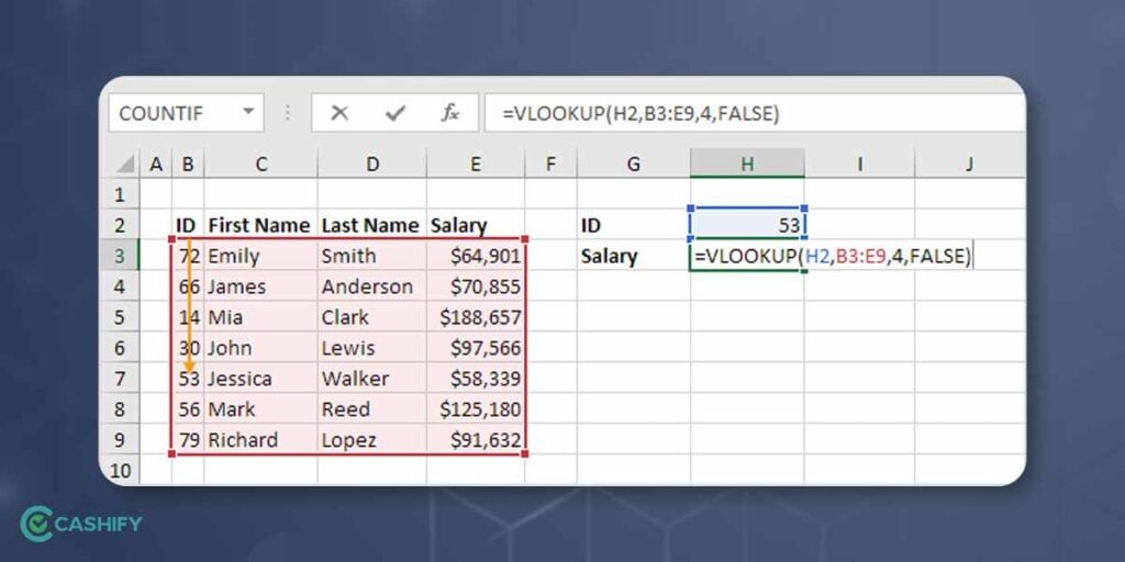
By simply typing in the formula followed by =VLOOKUP, you will be able to easily use the function. Here’s a quick look at the method:

• First and foremost, select the cell (H4 in our case)
• Here, type =VLOOKUP
• Then, double click on the command you just entered
• Select the cell where you will enter your search value (H3 in this case)
• After that, type (,)
• Now you have to mark the table range (let us take A1:F15)
• Type (,) again
• Then, you have to type the number of the column
• You will have to Type (,) again
• Right after, type in the the range (for TRUE use 1, for FALSE use 0)
• Hit the Enter button
• Lastly, specify the value in the selected cell for your Lookup_value (in our case H3 followed by the cell number)

Also read: Best Apps To Download Doctor Strange Wallpaper And Ringtone

You can Sell Laptop Online or Recycle Old Laptop with Cashify and get rewarded for it. If your laptop is causing way too many problems, it is probably time to consider these two options and upgrade to a new one!